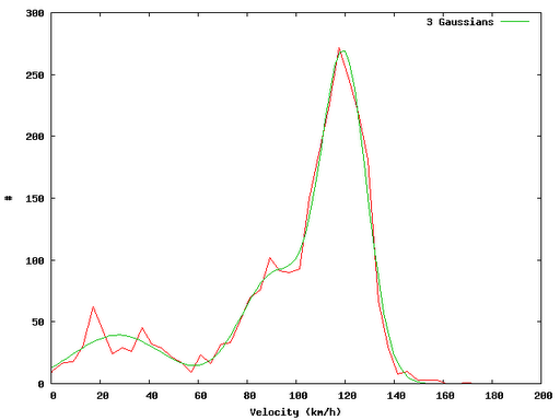
In this post I show a small example on how one can easily evaluate GPX track files using Perl and Gnuplot. The idea in brief: Read in GPX track infile.gpx and extract the velocity distribution. In a first approximation I have fitted gaussian distributions…

The calculation of distances between two points in WGS 84 coordinates is done using the approach given by Vincenty. There are methods with an accuracy of up to 10nm (geographiclib, interesting paper on this topic).

Code Snipplets

The code pieces listed below are extracts of what I have done. Do not expect the code to work - it shall only serve as an idea for you…

Perl Script

#!/usr/bin/perl

use Geo::Gpx;

use Data::Dumper;

use DateTime;

use GIS::Distance;

use Statistics::Lite qw(:all);

use POSIX;

my $gis = GIS::Distance->new();

$gis->formula (“Vincenty”);

my $fh = “infile.gpx”;

Extract vlat from GPX file

my $gpx = Geo::Gpx->new( input => $fh );

my $waypoints = $gpx->waypoints();

my $tracks = $gpx->tracks();

my $iter = $gpx->iterate_trackpoints(); #points();

my (@time, @lat, @lon, @ele);

while (my $pt = $iter->())

{

push (@time, $pt->{time}); # Linux Epoch time

push (@lat,$pt->{lat}); # WGS 84

push (@lon, $pt->{lon}); # WGS 84

push (@ele, $pt->{ele}); # meters

}

my %s_time = statshash (@time);

my %s_lat = statshash (@lat);

my %s_lon = statshash (@lon);

my %s_ele = statshash (@ele);

my $n = 1+$#time;

Velocities

my (@vlat, @dlateral_next, @vhor);

my $ms_kmh = 3.6;

for my $i (0..$n-2)

{

my $d = $gis->distance ($lat[$i],$lon[$i] => $lat[$i+1],$lon[$i+1]); 

my $dlateral = $d->meters(); # meters

my $dhorizontal = $ele[$i+1]-$ele[$i]; # meters

my $dt = $time[$i+1]-$time[$i]; # seconds

$dt > 0 or warn;

$dt > 0 or next;

my $vv = sqrt($dlateral**2)/$dt * $ms_kmh; 

my $hh = sqrt($dhorizontal**2)/$dt * $ms_kmh;

push (@vlat, $vv); # km/h

push (@vhor, $hh); # km/h

push (@dlateral_next, $dlateral); # meters

}

my %s_vlat = statshash (@vlat);

my %s_vhor = statshash (@vhor);

my %s_dlateral_next = statshash (@dlateral_next);

Distribution

sub distribution

{

my $nbins = floor(sqrt($n));

my $nsigma = 2;

my ($min, $max) = ($s_vlat{mean}-$nsigma$s_vlat{stddev}, $s_vlat{mean}+$nsigma$s_vlat{stddev});

my $d = ($max - $min) / $nbins;

my %hist;

for my $i (0..$nbins-1)

{

$hist{$i}{x} = $min+($i+.5)*$d;

}

for my $i (0..$n-2)

{

my $bin = floor(($vlat[$i]-$min)/$d);

$bin < 0 and warn;

$bin < 0 and $bin = 0;

$bin >= $nbins and warn;

$bin >= $nbins and $bin = $nbins-1;

$hist{$bin}{y} = $hist{$bin}{y}+1;

}

my $f_dist = “dist.txt”;

open (F_DIST, “>”.$f_dist);

for my $j (0..$nbins-1)

{

printf F_DIST “%d %f %f\n”, $j, $hist{$j}{x}, $hist{$j}{y};

}

}

distribution();

GnuPlot Fitting

f1(x) = p1*exp(-(x-m1)2/(2*s12))

f2(x) = p2*exp(-(x-m2)2/(2*s22))

f3(x) = p3*exp(-(x-m3)2/(2*s32))

m1=120

m2=80

m3=50

f(x) = f1(x)+f2(x)+f3(x)

fit f(x) “dist.txt” u 2:3 via p1,p2,p3,m1,m2,m3,s1,s2,s3

plot  ”dist.txt” u 2:3 w l,f(x)